Peeking inside the black-box

Introduction

The advance of machine learning (ML) has ushered in unprecedented capability across diverse domains, tackling the task of objective decision making given available data.^[1,2] Deep neural networks, in particular, have become a dominant paradigm, gaining popularity for handling complex tasks previously considered intractable for computational approaches.^[3] However, this success is often shadowed by a critical drawback: the inherent opacity of these models. Dubbed the “black-box” problem, the intricate, non-linear transformations with deep networks their decision-making processes inscrutable, hindering trust and accountability.^[4,5] This lack of transparency poses a significant impediment to the broader adoption of ML, especially in high-stakes applications (such as financial algorithms), where interpretability and robust parameter analysis are paramount.

To address this, researchers have employed various methods to illuminate the inner workings of complex ML architectures. While various post-hoc interpretability techniques offer valuable insights^[6,7], intrinsically interpretable models (predictive graphs) are a fundamentally more powerful tool. Piecewise linear neural networks (PWLNNs) present a compelling avenue, building upon the foundations of piecewise linearity - a concept with deep roots in mathematics and engineering - to enable the 3-dimensional representation of complex relationships.^[8,9]

This article builds upon the work of Jordan et al.^[10], Serra et al.^[11], and Pascanu et al.^[12], all focused on the academic principles of PWLNNs. Cheng^[13] moved beyond this, curating visual frameworks, but focuses on the artistic potential of this technique, limiting the possible technical improvements. This paper seeks to understand parameter influence, and ultimately optimise model design. Secondary advantages consist of increased trustworthiness as well as greater engagement for stakeholders with less technical backgrounds.

Theory

The interpretability of PWLNNS stem from their mathematical structure. Unlike smooth, continuously differentiable networks, these networks operate through a series of Rectified Linear Unit (ReLU) activation functions.^[14] Once multiple nodes are introduced, this architecture induces a set of polyhedral regions, within each of which the network's behaviour is government by a simple linear function.^[15,16]

Consider a standard feedforward neural network layer. In a PWLNN, each neuron \(j\) in layer \(l\) computes an output \(x_j^{(l)}\) from the input \(x^{(l-1)}\) from the preceding layer as: $$z_j^{(l)}=∑_iW_{ji}^{(l)}x_i^{(l-1)}+b_j^{(l)}$$ $$x_j^{(l)}=σ(z_j^{(l)})$$ Where \(W^{(l)}\) and \(b^{(l)}\) are the weight matrix and bias vector for layer \(l\), respectively, and \(σ(∙)\) is the ReLU activation function, defined as \(σ(z)=max(0,z)\). This seemingly simple non-linearity is the key to piecewise linearity. As highlighted in ^[17], the ReLU function introduces "kinks" at \(z=0\), dividing the input space into regions where the neuron is either "active" (outputting \(z\)) or "inactive" (outputting 0).

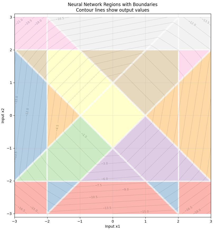
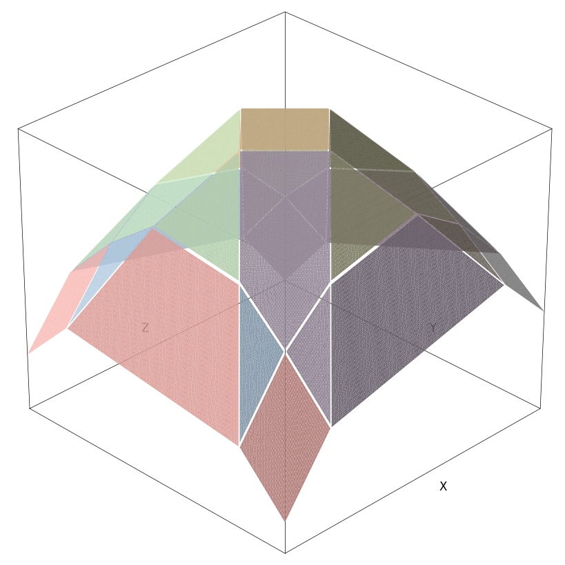
In figure 1, a single layer neural network is displayed in 2-dimensions, with each node's weighting and bias influencing the display. The graph is translucent with the output heights displayed topographically underneath. The layer can also be represented in 3-dimensions, as shown in figure 2:

Across multiple layers, these piecewise linear activations compound. As detailed in ^[18], the combined effect of ReLUs across all neurons and layers partitions the entire input space into hyperplanes. As such, the non-linear behaviour of neural networks emerge from stitching together these linear behaviours. Figure 3 illustrates a 2nd layer being added to the example neural net above:

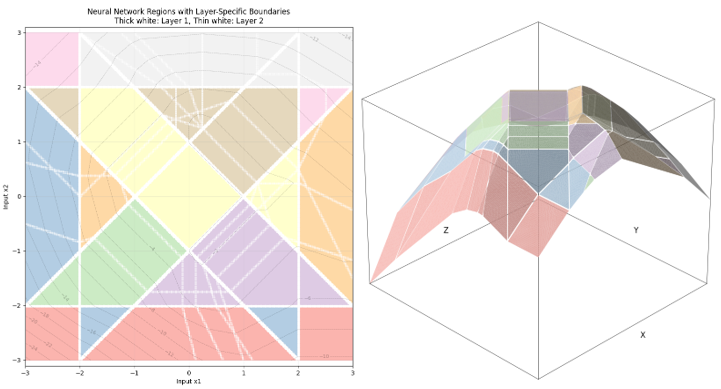
With added complexity, larger computational intensity is required to produce these results. Additionally, adding a second layer increases the number of regions that are not able to display graphically through having insufficient points for triangulation.^[19] Nonetheless, the 3d plot eloquently shows output upon inputs within the graph's boundaries.

Limitations

Whilst the representation of neural networks in this way is impressive, with it comes certain limitations. Most notable of which, to represent the complete model in 3-dimensional space, we are limited to 2 input variables. Many complex neural networks include many inputs, so this limits network complexity considerably. To rectify this constraint, the following options are present:

1. Utilise a fourth dimension (time) and create a timelapse to observe the effect of a third input.
2. Use dimensional reduction techniques to transmute greater numbers of inputs down to 2.

As a more comprehensive solution, option 2 is the clear step forward. Upon settling on this option, we are faced with 3 options: PCA, t-SNE, and UMAP. Principle Component Analysis (PCA) is the simplest, that transforms the data linearly as to capture the largest variation in the data. Meanwhile, t-distributed stochastic neighbour embedding (t-SNE) and Uniform Manifold Approximation and Projection (UMAP) are both more complex algorithms, and differ that t-SNE looks to emphasize local neighbourhood preservation whilst UMAP balances local preservation with global structure. Because of this, UMAP tends to scale more readily than t-SNE, and should be utilised for more complex situations. For clarity, all methods will be tested for the following neural net.

The Problem

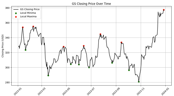
For a more complex example, identification of local minima and maxima for stocks will be used. In figure 4, historical 10-day minima and maxima are tracked for GS and the following values recorded:

• Volume - Represents the amount of share traded (both bought and sold) on a specific day.
• Normalised value - found via the following:$$Normalised\; value=\frac{CLOSE-LOW}{HIGH-LOW}$$
• 3-day regression coefficient - linear regression is formed over the past 3 days of closing prices. This represents the direction of the stock over the past 3 days.
• 5-day regression coefficient - Similar to above, instead using 5 days.
• 10-day regression coefficient - Similar to above, instead using 10 days.
• 20-day regression coefficient - Similar to above, instead using 20 days.

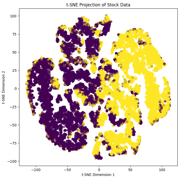
The above is collated for all stocks within the Dow Jones 30, and used as the model inputs. The outputs are either 0 or 1, depending whether correspond to a minima or maxima. The neural network then completes a binary classification task. With 6 input variables, the example cannot be represented via PWLNN. Instead, the three dimensional reduction techniques mentioned above are used to reduce the input variables for display purposes, with the objective of minimising accuracy sacrifice.

Method	Standard NN	PCA	t-SNE	UMAP
Numer of input variables	6	2	2	2
Accuracy	88.1%	81.0%	79.2%	85.6%
2-d projection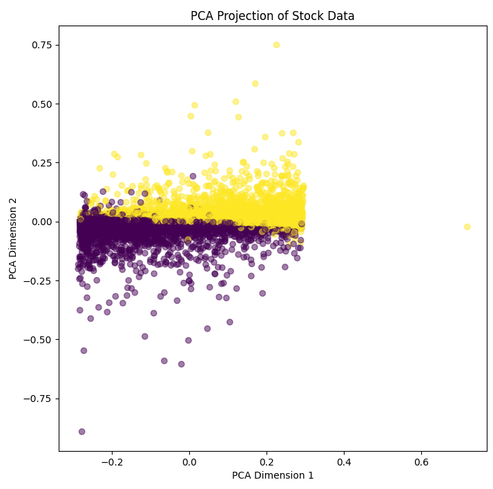

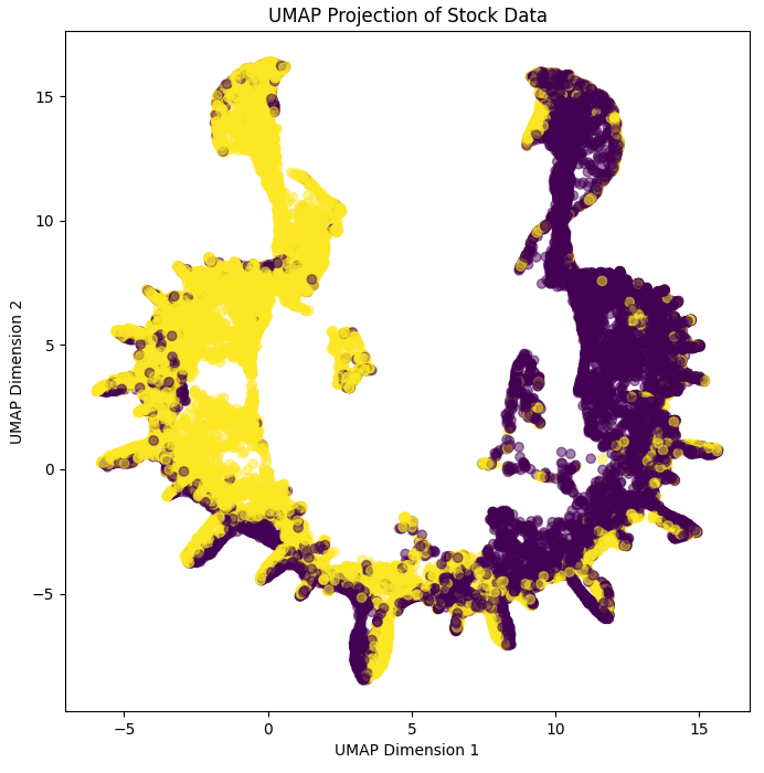Table 1 illustrates the varying effects of different dimensional reduction techniques. PCA draw the most definite line between maxima and minima, but fails to capture the intricacies of the data. t-SNE, focusing on local structure, captures the majority of local data relationships, but does so at the expense of global accuracy. This is evinced by the c. 9% drop in prediction accuracy over a test dataset. Meanwhile, UMAP seeks to maintain global parameter relationship, and doing so provides the highest prediction accuracy, only foregoing 2.5% accuracy on the unreduced inputs. See the 3-d projection of UMAP in figure 5 below:

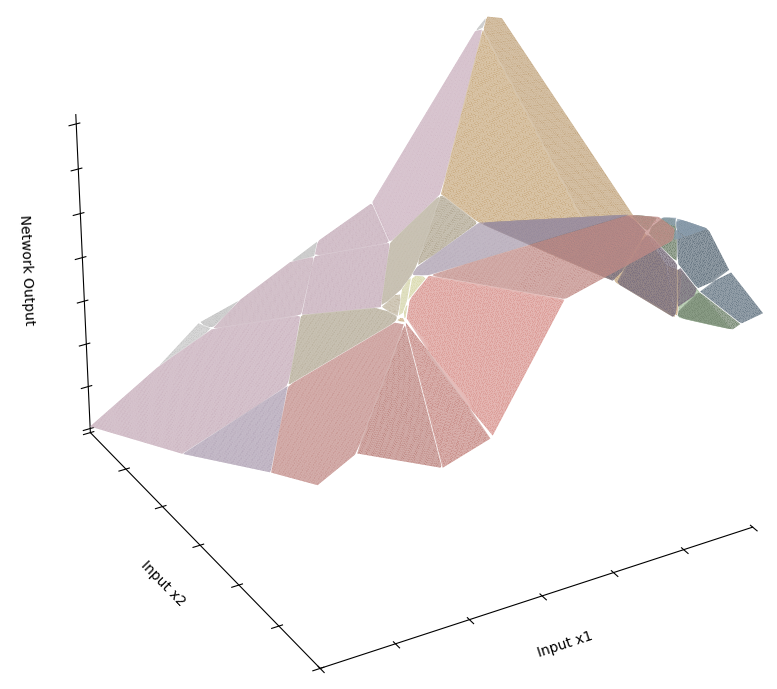
Figure 5 illustrates the neural net eloquently, however, as UMAP is a non-linear technique, no direct variable to variable mapping is possible, and we lose some understanding of how input variables affect the resulting output shape. As a binary classification model, we are hoping to see distinct minima and maxima, however with the complicated task posed above, this is not always possible. 2 maxima are represented in the graph, with the space in between producing values that are unhelpful/misleading for this exercise. To progress this further, we can repeat dimensional reduction differing the variables included. A combination of the resultant graph and Shapley Additive exPlanations (SHAP) can be used to explain model outputs more fully.

Worth noting, as mentioned in Cheng^[13], figure 5 shows that small ReLU networks become stuck in local minima, seen by the large number of intersections in the centre of the grid. To solve this, a leaky ReLU function can instead be used, although this is unnecessary for a grid of only 2 layers pictured above.

Conclusion

By leveraging the inherent piecewise linear nature of ReLU activation functions, we demonstrated the capability to represent neural network behaviour in a visually intuitive 3-dimensional space. This approach offers a significant advantage in demystifying the 'black-box' nature of complex models, potentially fostering greater trust and understanding amongst both technical and non-technical stakeholders.

Recognising the limitation of 3D visualisation to two input variables, we investigated dimensionality reduction techniques to extend the applicability of PWLNNs to higher-dimensional datasets. Our comparative analysis of PCA, t-SNE, and UMAP revealed UMAP as a particularly effective method for this purpose. UMAP demonstrated the best balance between preserving prediction accuracy and enabling meaningful 2-dimensional projections suitable for PWLNN visualisation, only sacrificing a marginal 2.5% accuracy compared to the full input model. While UMAP's non-linear nature introduces a trade-off by obscuring direct input-variable relationships, the resulting visualisations, as seen in Figure 5, still provide valuable qualitative insights into the model's decision boundaries and output landscape.

Future work should focus on refining dimensional reduction techniques specifically tailored for neural network visualization, potentially developing methods that better preserve the relationship between original input variables and their reduced representations. Additionally, exploring the effectiveness of these visualization approaches across different domains and model architectures would enhance their broader applicability. Whilst not utilised in this article, SHAP, a game theoretic approach to this problem, can be utilised alongside visualisation techniques to attain greater knowledge of input variable effects.

In conclusion, the graphical representation of neural networks through PWLNNs offers a promising avenue for improving model transparency, facilitating parameter analysis, and ultimately building trust in high-stakes applications. By making the complex decision boundaries of neural networks visually accessible, we take a significant step toward reconciling the powerful predictive capabilities of deep learning with the interpretability demands of critical domains.

References:

[1] LeCun, Y., Bengio, Y., & Hinton, G. (2015). Deep learning. Nature, 521(7553), 436-444.

[2] Jordan, M. I., & Mitchell, T. M. (2015). Machine learning: Trends, perspectives, and prospects. Science, 349(6245), 255-260.

[3] Goodfellow, I., Bengio, Y., & Courville, A. (2016). Deep Learning. MIT Press.

[4] Rudin, C. (2019). Stop explaining black box machine learning models for high stakes decisions and use interpretable models instead. Nature Machine Intelligence, 1(5), 206-215.

[5] Lipton, Z. C. (2018). The mythos of model interpretability. Communications of the ACM, 61(10), 36-43.

[6] Ribeiro, M. T., Singh, S., & Guestrin, C. (2016). "Why should I trust you?": Explaining the predictions of any classifier. Proceedings of the 22nd ACM SIGKDD International Conference on Knowledge Discovery and Data Mining, 1135-1144.

[7] Lundberg, S. M., & Lee, S. I. (2017). A unified approach to interpreting model predictions. Advances in Neural Information Processing Systems, 30.

[8] Montufar, G. F., Pascanu, R., Cho, K., & Bengio, Y. (2014). On the number of linear regions of deep neural networks. Advances in Neural Information Processing Systems, 27.

[9] Arora, R., Basu, A., Mianjy, P., & Mukherjee, A. (2018). Understanding deep neural networks with rectified linear units. International Conference on Learning Representations.

[10] Jordan, M. I., Ghahramani, Z., Jaakkola, T. S., & Saul, L. K. (1999). An introduction to variational methods for graphical models. Machine Learning, 37(2), 183-233.

[11] Serra, T., Tjandraatmadja, C., & Ramalingam, S. (2018). Bounding and counting linear regions of deep neural networks. International Conference on Machine Learning, 4558-4566.

[12] Pascanu, R., Montufar, G., & Bengio, Y. (2013). On the number of response regions of deep feed forward networks with piece-wise linear activations. arXiv preprint arXiv:1312.6098.

[13] Cheng, C. H. (2018). A neural network visualization framework for high-dimensional datasets. IEEE Transactions on Visualization and Computer Graphics, 24(1), 923-932.

[14] Nair, V., & Hinton, G. E. (2010). Rectified linear units improve restricted Boltzmann machines. Proceedings of the 27th International Conference on Machine Learning, 807-814.

[15] Hanin, B., & Rolnick, D. (2019). Complexity of linear regions in deep networks. International Conference on Machine Learning, 2596-2604.

[16] Raghu, M., Poole, B., Kleinberg, J., Ganguli, S., & Dickstein, J. S. (2017). On the expressive power of deep neural networks. International Conference on Machine Learning, 2847-2854.

[17] He, K., Zhang, X., Ren, S., & Sun, J. (2016). Deep residual learning for image recognition. Proceedings of the IEEE Conference on Computer Vision and Pattern Recognition, 770-778.

[18] Zhang, C., Bengio, S., Hardt, M., Recht, B., & Vinyals, O. (2017). Understanding deep learning requires rethinking generalization. International Conference on Learning Representations.

[19] Balestriero, R., & Baraniuk, R. (2018). A spline theory of deep learning. International Conference on Machine Learning, 374-383.